What is Variance Analysis? | Cost Accounting

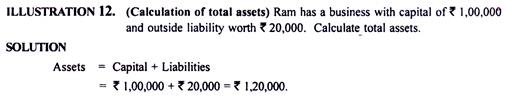
Get the answer of: What is Variance Analysis?

‘Variance’ is the difference between planned, budgeted or standard cost and actual costs and similarly in respect of revenues. This should not be confused with the statistical variance which measures the dispersion of a statistical population.

‘Variance Accounting’ is a technique whereby the planned activities of an undertaking are quantified in budgets, standard costs, standard selling prices and standard profit margins, and the differences between these and the actual results are compared. The procedure is to collect, compare, comment and correct.

‘Variance Analysis’ is the analysis of variances arising in a standard costing system into their constituent parts. It is the analysis and comparison of the factors which have caused the differences between predetermined standards and actual results, with a view to eliminating inefficiencies.

Variance analysis highlights areas of strengths and weaknesses, but doesn’t indicate what action, if any, should be taken. A manager must be able to correctly interpret the significance of variances before he can initiate control action. All planning is based on estimates (e.g., of prices, costs, volumes) and actual outcomes will rarely be precisely in line with these estimates. Some variation is inevitable.

Variances obtained under standard costing system have to be reported to management for taking remedial steps. Before taking any action, the management must try to know the causes of such variances. In a business organization, control is a relative rather than absolute concept.

Seldom, the management will attempt to maintain absolute control. Control is justified only to the extent that it produces values and the excess control is not suggested where the cost of control exceeds the values it produces. Thus in some instances exercising little control may be the best policy.

For understanding of the ‘variance analysis’ topic, variances are classified into the following:

(i) Material variances,

(ii) Labour variances,

(iii) Variable overhead variances,

(iv) Fixed overhead variances,

(v) Sales variances, and

(vi) Profit variances.

Each of these variances are discussed elaborately in the following paragraphs:

(i) Material Variances:

For the purpose of material variance analysis, the following two types of standards need be fixed.

1. Material Price Standards:

Price factor is controlled by external factors. If the price changes during the period due to inflation, raise in prices of controlled items like cement, steel, etc., there is going to be wide variations.

Material prices are fixed keeping in mind the terms of contract of purchases, nature of items and other relevant factors. Some organizations have regular system of purchases (rate contract) for the whole period/year at predetermined price irrespective of the prevalent market rates.

2. Material Quantity Standards:

Quantity usage standards are set on the basis of various test runs and guidelines provided by R&D department or Engineering department and specifications on the basis of past experience. The standards should also take into consideration allowances for acceptable level of waste, spoilage, shrinkage, seepage, evaporation, leakage, etc.

3. Material Cost Variance:

The material cost variance is also called ‘material total variance’ is the difference between standard direct material cost of actual production and the actual cost of direct material.

(Standard units x Standard price) – (Actual units x Actual price)

or Standard cost of material – Actual cost of material used

4. Material Price Variance:

The material price variance is the difference between the standard price and the actual purchase price for each unit of material multiplied by the actual quantity of material purchased. It is preferable to base the price variance on the actual quantity of material purchased and not on the actual quantity used in order that price variances can be reported for control purposes.

Actual quantity (Standard price p.u. – Actual price p.u.)

5. Material Usage Variance:

The material usage variance is the difference between the actual quantity of material used and the standard quantity of material that should be used for actual production, multiplied by the standard price per unit of material.

Standard price p.u. (Standard quantity – Actual quantity)

Material usage variance is further segregated into (a) Material mix variance, and (b) Material yield variance.

6. Material Mix Variance:

If a process uses several different materials which could be combined in a standard proportion, a mix variance can be calculated which shows the effect on cost of variances from the standard proportion. There are two recognized ways of calculating this mix variance.

Some authorities regard the variance as a subset of the usage variance but others treat it as part of the price variance. If the mix variance is treated as a subset of the usage variance, then the material mix variance is the difference between the total quantity in standard proportion priced at the standard price and the actual quantity of material used priced at the standard price.

Material Mix Variance

Standard price (Revised standard quantity – Actual quantity)

Revised Standard Quantity

(Total quantity of actual mix/Total quantity of standard mix) x Standard quantity

7. Material Yield Variance:

Apart from operator or machine performance, output quantities produced are often different to those planned, e.g., this arises in chemical plants where plant should produce a given output over a period for a given input but the actual output differs for a variety of reasons. Material yield variance is the difference between the standard yield of the actual material input and the actual yield, both valued at the standard material cost of the product.

Standard cost p.u. (Standard output for actual mix – Actual output)

(ii) Labour Variances:

Normally it is taken that labour is a variable cost but at times it becomes fixed cost as it is not possible to remove or retrench in case of fall/stoppage in production.

Labour Rate Standard and Grades of Labour:

This is basically dependent on the agreement with the labour unions or rate prevalent in the particular area or industry.

1. Labour Efficiency Standard:

The labour (quantities) efficiency means the number of hours that the appropriate grade of worker will take to perform the necessary work. It is based on actual performance of worker or group of workers possessing average skill and using average effort while performing manual operations or working on machine under normal conditions. The standard time is fixed keeping in mind the past performance records or work study. This is on the basis that is acceptable to the worker as well as the management.

2. Labour Cost Variance:

The labour cost variance is also called’ labour total variance’ is the difference between the standard direct labour cost and the actual direct labour cost incurred for the production achieved.

(Standard labour hours produced x Standard rate per hour) – (Actual direct labour hours x Actual rate per hour)

or Standard cost for actual output – Actual cost

3. Labour Rate Variance:

The labour rate variance is the difference between the actual direct labour rate per hour and the standard direct labour rate per hour, multiplied by the actual hours paid, i.e., the rate per hour paid to the direct labour force more or less than standard use of higher/lower grade of skilled workers than planned or wage inflation causes this variance.

Actual time (Standard rate – Actual rate)

4. Labour Efficiency Variance:

The labour efficiency variance is the difference between the actual hours taken to produce the actual output and the standard hours that this output should have taken, multiplied by the standard rate per hour. The possible cause for this variance is due to use of higher/lower grade of skilled workers than planned or the quality of material used, errors in allocating time to jobs.

Standard rate (Standard time for actual output – Actual time)

The labour efficiency variance can be segregated into the following:

5. Labour Mix Variance:

The labour mix variance arises due to change in composition of labour force.

Labour Mix Variance

Standard rate (Revised standard time – Actual time)

Revised Standard Time

Total actual time/Total standard time x Standard time

6. Labour Yield Variance:

The labour yield variance arise due to the difference in the standard output specified and the actual output obtained.

Standard cost p.u. (Standard output for actual time – Actual output)

7. Idle Time Variance:

The idle time variance represents the difference between hours paid and hours worked, i.e., idle hours multiplied by the standard wage rate per hour. This variance may arise due to illness, machine breakdown, holdups on the production line because of lack of material.

Idle hours x Standard rate

8. Net Efficiency Variance:

This variance is calculated after deducting idle hours from actual hours. The efficiency variance less idle time variance is called ‘net efficiency variance’.

Standard rate ( Standard time for actual output – Actual time worked)

or Standard rate (Standard time – Actual hours paid – Idle time)

Illustration 1:

100 skilled workmen, 40 semiskilled workmen and 60 unskilled workmen were to work for 30 weeks to get a contract job completed. The standard weekly wages were Rs. 60, Rs. 36 and Rs. 24 respectively. The job was actually completed in 32 weeks by 80 skilled, 50 semiskilled and 70 unskilled workmen who were paid Rs. 65, Rs. 40 and Rs. 20 respectively as weekly wages.

Find out the labour cost variance, labour rate variance, labour mix variance and labour efficiency variance.

Solution:

Basic Data for Calculation of Labour Variances:

 

 

 

 

 

 

Calculation of Labour Variances:

(1) Direct Labour Cost Variance

Std. cost for actual output – Actual cost

= 2,75,200- 2,66,400 = Rs. 8,800 (A)

(2) Direct Labour Rate Variance Actual time (Std. rate – Actual rate)

Skilled = 2,560(60- 65) = Rs. 12,800 (A)

Semiskilled = 1,600(36 – 40) = Rs. 6,400 (A)

Unskilled = 2,240 (24 – 20) = Rs. 8.960 (F) = Rs. 10,240 (A)

(3) Direct Labour Efficiency Variance

Std. rate (Std. time for actual output – Actual time)

Skilled = 60(3,000 – 2,560) = Rs. 26,400 (F)

Semiskilled = 36(1,200 – 1,600) = Rs. 14,400 (A)

Unskilled = 24 (1,800 – 2,240) = Rs. 10,560 (A) = Rs. 1,440 (F)

Direct Labour Efficiency Variance can be further analyzed into:

(a) Direct Labour Mix Variance

Std. rate (Revised std. time – Actual time)

Skilled = 60 (3,200 – 2,560) = Rs. 38,400 (F)

Semiskilled = 36 (1,280 – 1,600) = Rs. 11,520 (A)

Unskilled = 24 (1,920 – 2,240) = Rs. 7.680 (A) = Rs. 19,200 (F)

Revised std. time

Skilled =6,400/6,000 x 3,000 = 3,200

Semi-Skilled = 6,400/6,000 x 1,200 = 1,280

Unskilled = 6,400/6,000 x 1,800 = 1,920

(b) Direct Labour Revised Efficiency Variance

Std. rate (Std. time for actual output – Revised std. time)

Skilled = 60(3,000 – 3,200) = Rs. 12,000 (A)

Semiskilled =36 (1,200 – 1,280) = Rs. 2,880 (A)

Unskilled =24(1,800 – 1,920) = Rs. 2.880 (A) = Rs. 17,760 (A)

 

 

 

 

 

(iii) Variable Overhead Variances:

For fixation of costs for overheads, a survey of overheads will be necessary and with the data available for budgetary control, the overheads will be charged to various cost centres/products etc. on the basis of standard costs. For this, after dividing the overheads into fixed and variable the calculation of standard overhead rate for each cost centre/product is done.

The number of hours representing the capacity to manufacture is to be reduced by various idle facilities, etc. The choice of method of absorption (direct wage rate or machine hour) will depend upon the circumstances. The main object is to establish a normal overhead rate based on total factory overhead at normal capacity volume.

1. Variable Overhead Cost Variance:

The variable overhead cost variance represents the difference between the standard cost of variable overhead allowed for actual output and the actual variable overhead incurred during the period. The variance represents the under absorption or over absorption of variable overheads.

(Actual output x Standard variable overhead rate p.u.) – Actual variable overhead cost

or (Standard hours for actual output x Standard variable overhead rate per hour) – Actual variable overhead cost

2. Variable Overhead Expenditure Variance:

It is the difference between the actual variable overhead rate per hour and the standard variable overhead rate per hour multiplied by the actual hours worked. The actual hours worked must be used not the actual hours paid because the latter may include idle time and it is usually assumed that variable overhead will not be recovered in idle time.

(Standard variable overhead rate x Budgeted output) – Actual variable overheads

or (Standard hours for budgeted output x Standard variable overhead rate per hour) – Actual variable overheads

or Budgeted variable overheads – Actual variable overheads

3. Variable Overhead Efficiency Variance:

The variable overhead efficiency variance is calculated by taking the difference in standard output and actual output multiplied by the standard variable overhead rate.

Standard variable overhead rate (Standard output – Actual output)

Illustration 2:

The budgeted variable overheads for March are Rs. 3,840. Budgeted production for the month is 38,400 units. The actual variable overheads incurred were Rs. 3,830 and actual production was 38,640 units. Calculate variable production overhead variance.

Solution:

Working Notes:

Standard Variable Overhead p.u.

Budgeted variable overhead/Budgeted production = Rs. 3,840/38,400 =Re. 0.10

Budgeted production 38,400 units

Total Standard Variable Overhead

= Actual quantity x Std. variable overhead p.u.

= 38,640 units x Re. 0.10 = Rs. 3,864

Variable Production Overhead

= Standard variable overhead – Actual variable overhead

= Rs. 3,864 – Rs. 3,830 = Rs. 34 (F)

(iv) Fixed Overhead Variances:

Fixed overhead represents all items of expenditure which are more or less remain constant irrespective of the level of output or the number of hours worked.

The fixed overheads variances are classified as follows:

1. Fixed Overhead Cost Variance:

The fixed overhead cost variance represents the under/over absorbed fixed production overhead in the period. This under/over absorbed overhead may be due to differences between actual and budgeted fixed overheads, i.e., expenditure variances, and/or differences between the actual and budgeted levels of activity i.e., volume variances.

(Actual output x Standard fixed overhead rate p.u.) – Actual fixed overheads

or (Standard hours for actual output x Standard fixed overhead rate per hour) – Actual fixed overheads

or Recovered fixed overheads – Actual fixed overheads

2. Fixed Overhead Expenditure Variance:

This variance is also called ‘budget variance’, obtained by comparing the total fixed overhead cost actually incurred against the budgeted fixed overhead cost.

Budgeted fixed overheads – Actual fixed overheads

Fixed Overhead Volume Variance:

The volume variance is computed by taking the difference between overhead absorbed on actual output and those on budgeted output.

(Actual output x Standard rate) – Budgeted fixed overheads

or Standard rate (Actual output – Budgeted output)

or Standard rate per hour (Standard hours produced – Budgeted hours)

3. Fixed Overhead Efficiency Variance:

The efficiency variance arise due to the difference between budgeted efficiency to production and the actual efficiency is achieved.

Standard rate (Actual output in units – Standard output in units)

or Standard rate per hour (Actual hours worked – Standard hours for actual output)

4. Fixed Overhead Capacity Variance:

The capacity variance represents the part of volume variance which arise due to working at higher or lower capacity than standard capacity.

Standard rate (Budgeted quantity – Standard quantity)

5. Revised Fixed Overhead Capacity Variance:

The revised capacity variance is calculated as follows:

Standard fixed overhead rate (Revised budgeted quantity – Standard quantity)

6. Fixed Overhead Calendar Variance:

The calendar variance arise due to the volume variance which is due to the difference between the number of working days anticipated in the budget period and the actual working days in the period to which the budget is applied.

Standard fixed overhead rate (Budgeted quantity – Revised budgeted quantity)

(v) Sales Variances:

All of the variances discussed previously have been concerned with costs; the effects on profits due to adverse or favourable variances affecting direct materials, direct labour or overheads. Some companies calculate cost variances only, but to obtain the full advantages of standard costing, it is required to calculate sales variances.

Sales variances affect a business in terms of changes in revenue: changes which have been caused either by a variation in sales quantities or in sales prices.

There are two distinctly separate systems of calculating sales variances, which show the effect of a change in sales as regards:

(i) Sales margin variance (on the basis of profit), and

(ii) Sales value variance (on the basis of turnover).

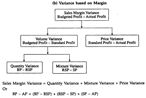
1. Sales Variances Based on Profit:

The sales variances based on profit are also called ‘sales margin variances’ which indicated the deviation between actual profit and standard or budgeted profit:

2. Total Sales Margin Variance:

This variance takes into account the difference between actual profit and standard or budgeted profit.

Actual profit – Budgeted profit

or (Actual quantity of sales x Actual profit p.u.) – (Budgeted quantity of sales x Budgeted profit p.u.)

3. Sales Price Variance:

The price variance is the difference between standard price of the quantity of sales effected and the actual price of those sales.

Actual quantity of sales (Actual profit p.u. – Standard profit p.u.)

or (Actual quantity of sales x Standard price) – (Actual quantity of sales x Actual price)

4. Sales Volume Variance:

It represents the difference between the actual units sold and the budgeted quantity multiplied by either the standard profit per unit or the standard contribution per unit. In absorption costing standard profit per unit is used, but in marginal costing, standard contribution per unit must be used.

Standard profit p.u. (Actual quantity of sales – Standard quantity of sales)

or Standard profit on actual quantity of sales – Standard profit on standard quantity of sales

Sales volume variance can be further segregated into (a) Sales mix variance and (b) Sales quantity variance as given below:

5. Sales Mix Variance:

The sales mix variance arises when the company manufactures and sells more than one type of product. This variance will be due to variation of actual mix and budgeted mix of sales.

Standard profit p.u. (Actual quantity of sales – Standard proportion for actual sales)

Or Standard profit – Revised standard profit

6. Sales Quantity Variance:

The sales quantity is the difference between the budgeted profit on budgeted sales and expected profit on actual sales.

Standard profit p.u. (Standard proportion for actual sales – Budgeted quantity of sales)

or Revised Standard Profit – Budgeted Profit

or Budgeted margin p.u. on budgeted mix (Total actual quantity – Total budgeted quantity)

Illustration 3:

Majestic Auto Ltd. is manufacturing and selling three standard products. The company has a standard cost system and analyses the variances between the budget and the actual periodically.

The summarized working result for 2008-09 were as follows:

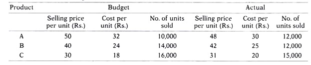
(a) Calculate the variance in profit during the period.

(b) Analyze the variance in profit into:

(i) Sales price variance

(ii) Sales volume variance

(iii) Cost variance

(iv) Sales margin quantity variance

(v) Sales margin mix variance.

Solution:

Working Notes:

(1) (a) Actual Margin Per Unit

Actual sales price per unit – Standard cost per unit

A = Rs. 48-Rs. 32 = Rs. 16

B = Rs. 42 – Rs. 24 = Rs. 18

C = Rs. 31 – Rs. 18 = Rs. 13

(b) Budgeted Margin Per Unit

Budgeted sales price per unit – Standard cost per unit

A = Rs. 50 – Rs. 32 = Rs. 18

B = Rs. 40 – Rs. 24 = Rs. 16

C = Rs. 30 – Rs. 18 = Rs. 12

(2) (a) Actual Profit

= Actual quantity of units sold x Actual margin per unit

(b) Budgeted Profit

= Budgeted quantity of units sold x Budgeted margin per unit

(3)(a) Budgeted Margin Per Unit on Actual Mix

(18 x 12,000) + (16 x 12,000) + (12 x 15,000)/39,000

2,16,000 + 1,92,000 + 1,80,000/39,000 = Rs. 15.077 p.u.

(b) Budgeted Margin Per Unit on Budgeted Mix

(18 x 10,000) + (16 x 14,000) + (12 x 16,000)/40,000

1,80,000 + 2,24,000 + 1,92,000/40,000 = Rs. 14.90 p.u.

Calculation of Sales Variances:

(1) Total Sales Margin Variance:

Actual profit – Budgeted profit

= Rs. 6,03,000 – Rs. 5,96,000 = Rs. 7,000 (F)

(2) Sales Margin Price Variance:

Actual qty. (Actual margin per unit – Budgeted margin per unit)

A = 12,000(16 – 18) = 24.000 (A)

B = 12,000(18 – 16) = 24.000 (F)

C = 15,000(13 – 12) = 15.000 (F)

= Rs. 15.000(F)

(3) Sales Margin Volume Variance:

Budgeted margin per unit (Actual qty. – Budgeted qty.)

A =18(12,000 – 10,000) = 36.000 (F)

B = 16 (12,000 – 14,000) = 32,000 (A)

C = 12 (15,000 -16,000) = 12,000 (A)

= Rs. 8,000 (A)

The sales margin volume variance can be further segregated into the following:

(4) Sales Margin Mix Variance:

Total actual quantity (Budgeted margin p.u. on actual mix – Budgeted

margin p.u. on budgeted mix)

= 39,000 (15.077 – 14.90) = Rs. 6,900 (F)

(5) Sales Margin Quantity (Sub-volume) Variance:

Budgeted margin p.u. on budgeted mix (Total actual qty. – Total budgeted qty.)

= 14.90 (39,000 – 40,000) = Rs. 14,900 (A)

 

 

 

 

 

7. Sales Variances Based on Turnover:

The sales variances based on turnover are classified as follows:

Sales Value Variance:

(Actual quantity x Actual selling price) – (Standard quantity x Standard selling price)

Sales Price Variance:

Actual quantity (Actual selling price – Standard selling price)

Sales Volume Variance:

Standard selling price (Actual quantity of sales – Standard quantity of sales)

Sales Mix Variance:

Standard value of actual mix – Standard value of revised standard mix

Sales Quantity Variance:

Standard selling price per unit (Standard proportion for actual sales quantity – Budgeted quantity of sales)

or Revised standard sales value – Budgeted sales value

Illustration 4:

The standard cost data of three products X, Y and Z manufactured by a company are given below together with the budgeted sales and unit selling prices for 2008-09:

You are required to determine:

(a) The budgeted and the actual profit for 2008-09

(b) The variance in profit analyzed into (i) Cost variance, (ii) Sales price variance, (iii) Sales value variance.

Solution:

Basic Data:

 

 

 

 

 

 

 

 

 

 

Calculation of Variances:

 

 

 

 

 

 

 

 

 

 

 

 

 

 

 

 

(vi) Profit Variances:

The profit variances are classified as follows:

Formulas:

Profit Value Variance:

Budgeted profit – Actual profit

Profit Price Variance:

Actual quantity (Standard rate of profit – Actual rate of profit)

Profit Volume Variance:

Standard rate of profit (Budgeted quantity – Actual quantity)

Profit Mix Variance:

Revised standard profit – Standard profit

Profit Quantity Variance:

Budgeted profit – Revised standard profit

 Illustration 5:

The standard wages per unit is based on 9,600 hours for the above period at the rate of Rs. 3.00 per hour. 6,400 hours were actually worked during the above period, and in addition, wages for 400 hours were paid to compensate for idle time due to breakdown of a machine, and overall wage rate was Rs. 3.25 per hour.

You are required to compute the following variances with appropriate workings:

a) Direct material cost variance,

b) Material price variance,

c) Material usage variance,

d) Direct labour cost variance,

e) Wage rate variance,

f) Labour efficiency variance,

g) Idle time variance,

h) Variable expenses variance,

i) Fixed expenses expenditure variance,

j) Fixed expenses volume variance,

k) Fixed expenses capacity variance,

l) Fixed expenses efficiency variance, and 

m) Total cost variance.

Solution:

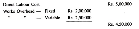
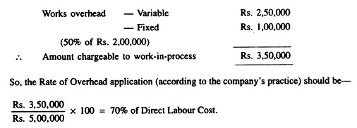
Working Notes:

1. Calculation of Standard and Actual Cost of Material for Actual Output i.e., 3,500 units

 

 

 

 

2. Standard and Actual Labour Costs for Actual Output of3,500 units:

 

 

 

 

 

 

 

 

 

 

 

 

 

 

 

 

 

 

 

 

(i) Direct Material Variances:

(a) Direct Material Cost Variance

Std. cost – Actual cost

= 1,75,000 – 1,89,000 = Rs. 14,000 (A)

(b) Material Price Variance

Actual qty. (Std. price – Actual price)

= 3,600 (50 – 52.50) = Rs. 9,000 (A)

(c) Material Usage Variance

Std. price (Std. qty. – Actual qty.)

= 50(3,500- 3,600) = Rs. 5,000 (A)

(ii) Labour Variances:

(d) Direct Labour Cost Variance

Std. cost – Actual cost

= 21,000 – 22,100 = Rs. 1,100 (A)

(e) Wage Rate Variance

Actual hours paid (Standard rate – Actual rate)

= 6,800 (3 – 3.25) = Rs. 1,700 (A)

(f) Labour Efficiency Variance

Std. rate per hour (Std. hours – Actual hours worked)

= 3 (7,000 – 6,400) = Rs. 1,800 (F)

(g) Idle Time Variance

Std. rate per hour (Labour hours worked – Labour hour paid)

= 3 (6,400 – 6,800) = Rs. 1,200 (A)

(iii) Overhead Variances:

(h) Variable Expenses Variance

Std. variable expenses – Actual variable expenses

= 70,000 – 62,000 = Rs. 8,000 (F)

(i) Fixed Expenses Expenditure Variance

Budgeted fixed expenses – Actual fixed expenses

= 1,92,000 – 1,88,000 = Rs. 4,000 (F)

(j) Fixed Expenses Volume Variance

Std. fixed expenses rate per unit x (Actual output – Budgeted output)

= 40 (3,500 – 4,800)= Rs. 52,000 (A)

(k) Fixed Expenses Capacity Variance

Std. fixed expenses rate per hour x (Actual capacity hours – Budgeted capacity hours)

= 20(6,800-9,600) = Rs. 56,000 (A)

(l) Fixed Expenses Efficiency Variance

Std. fixed expenses rate per hour x (Std. hours for actual output – Actual hours)

= 20 (7,000-6,800) = Rs. 4,000 (F)

(m) Total Cost Variance

Total std. cost – Total actual cost

= (3,500 x 116)-4,61,100 = Rs. 55.100(A)

 

 

 

 

 

 

 

 

 

Benefits and Problems of Variance Analysis:

The segregation of traditional variances into those which are due to planning deficiencies and those which are due to controllable factors is probably not widely used, but it does have the following benefits:

(a) It makes standard costing and variance analysis more realistic and meaningful in volatile and changing conditions.

(b) Operational variances provide an up-to-date guide to current levels of operating efficiency as the standards have been recalculated using up-to-date information.

(c) Having up-to-date standards and, therefore, more meaningful variances is likely to make the standard costing system more acceptable and to have a positive effect on motivation.

(d) It emphasizes the importance of the planning function in the preparation of standards and helps to identify planning deficiencies.

(e) The calculation of such variances provides a systematic method of reviewing standards and the assumptions contained within them.

The following are the problems in using such variances:

(a) There is an element of subjectivity in determining after the event (i.e., ex-post) what is a realistic price. This makes the allocation between planning and operational causes a subjective matter susceptible to political pressures.

(b) There is undeniably more clerical and managerial time involved in continually establishing up-to-date standards and calculating additional variances.

(c} Where the planning and operating functions are carried out in the same responsibility centre there is likely to be pressure to put as much as possible of the total variance down to outside, uncontrollable factors rather than internal, controllable actions. However, these pressures exist in the interpretation of any type of variance.